Skip to a subsection :
- ANNOTATIONS
- CLEAR
- PLOT WITH DIFFERENT SCALE
- MOSAIC
- GRIDSPEC
- PATCHES
- TEXT ALIGMENT
- IMSHOW
- QUIVER, CONTOUR, CONTOURF
- LIGHTSOURCE
- SUBMODULES, TOOLKITS
- SHAPES ON FIGURE
- CHANGING SETTINGS WITH RCPARAMS
ANNOTATIONS
plt.annotate : places an annotation on the currently active subplot. It may not work as expected if you have multiple subplots. ax.annotate : places an annotation to a specific subplot within a figure. This method is more precise and flexible.
import matplotlib.pyplot as plt
ax.annotate('this annotation can be split\n accross two lines ', xy = (2500, 1000), color = 'white', fontsize = '40')
CLEAR
plt.clf() : completely clears the active figure. Use it when you want to create a new empty figure from scratch. It removes all subplots, axes, and any other graphical elements created in the figure. plt.cla() : only clears the axes of the active figure. Use it when you want to reuse the same figure but clear any plots present on the current axis ax.clear() : clears all graphical elements on the axis specified by the ax variable. Use it when working with specific subplots or axes within a complex figure
PLOTS WITH DIFFERENT SCALES
twinx() : allows you to overlay two different datasets with different scales
x = np.linspace(-10, 10, 200)
y1 = np.sin(x)
y2 = np.exp(x)
fig,ax1 = plt.subplots()
ax1.plot(x,y1, color='blue')
ax2 = ax1.twinx()
ax2.plot(x,y2, color='green')
plt.show()
MOSAIC
twinx() : allows you to overlay two different datasets with different scales
mos = [['A','A','E'],
    ['B','B','E']]
fig, axs = plt.subplot_mosaic(mos)
plt.tight_layout()
x = np.linspace(-10,10,100)
y1 = np.sin(x)
y2 = np.cos(x)
y3 = x * np.exp(x)
ax = axs['A']
ax.plot(x,y1, linewidth = 3, color = 'blue')
ax = axs['B']
ax.plot(x,y2, linewidth=3 , color = 'green')
ax = axs['E']
ax.plot(x,y3, linewidth= 4,color = 'red')
for ax_name in axs:
	ax = axs[ax_name]
	ax.set_title(str(ax_name))
plt.show()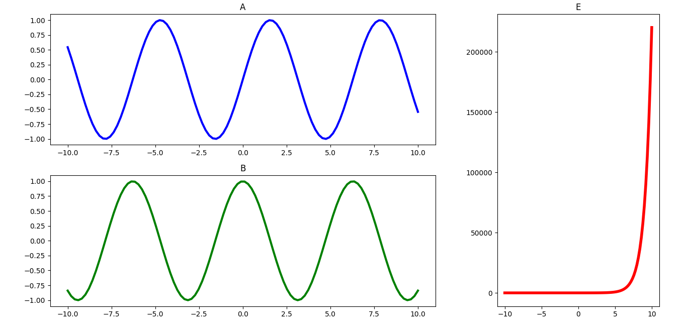
GRIDSPEC
Gridspec allows for arranging a set of graphs on a grid, which can simplify controlling the spacing between them. In this example, such a grid is created to represent an ellipse with varying parameters.
from matplotlib import pyplot as plt
import numpy as np
fig = plt.figure(figsize=(10,10))
fig.suptitle('Ellipses',color='black',fontsize=30)
rows,cols=5,5
gs = fig.add_gridspec(rows, cols, hspace=0.1, wspace=0.2)
t = np.linspace(0, 2 * np.pi, 100)
index = 0
for row in range(rows):
    for col in range(cols):
        ax = fig.add_subplot(gs[row, col])
        ax.set(xticks=[], yticks=[])
        ax.set_aspect('equal')
        ax.set_xlim(-5,5)
        ax.set_ylim(-5,5)
        a = 1 + index/10
        b = 3
        x = a*np.cos(t)
        y = b*np.sin(t)
        ax.plot(x,y)
        index+=1
plt.show()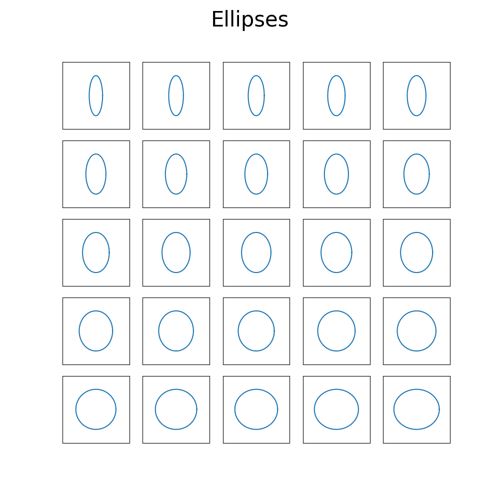
PATCHES
Patches are shapes that can be added to plots or figures : rectangles, circles, polygons, and other elements. Most of these shapes can be filled or left unfilled based on your preference. Here are some quick pointers on coordinates to help complete these examples. The coordinates provided as tuples represent the coordinates of
- the lower-left corner for the rectangle
- the center coordinates for the ellipse and the regular polygon.
import matplotlib.pyplot as plt
import matplotlib.patches as patches

fig, ax = plt.subplots()
circle = patches.Circle((2, 4), 1, fill=False, color='blue', linewidth=2)
arc = patches.Arc((1, 1), 2, 2, theta1=0, theta2=90, color='red', linewidth=2)
rectangle = patches.Rectangle((6, 6), 4, 2, fill=False, color='green', linewidth=3)
ellipse = patches.Ellipse((4, 3), width=2, height=1, angle=45, fill=False, color='purple', linewidth=2)
wedge = patches.Wedge(center=(7, 3), r=2, theta1=45, theta2=270, fill=True, color='orange', linewidth=2)
polygon_coords = [(0.2, 0.2), (0.4, 0.4), (0.6, 0.2), (0.6, 4), (0.2, 2)]
polygon = patches.Polygon(polygon_coords, closed=True, fill=False, color='navy', linewidth=2)
regular_polygon = patches.RegularPolygon((5, 7), numVertices=6, radius=2, orientation=0.0, fill=False, color='blue', linewidth=2)
arrow = patches.Arrow(x=1, y=8, dx=4, dy=1.5, width=0.5, color='red')

ax.add_patch(arc)
ax.add_patch(circle)
ax.add_patch(rectangle)
ax.add_patch(ellipse)
ax.add_patch(wedge)
ax.add_patch(polygon)
ax.add_patch(regular_polygon)
ax.add_patch(arrow)
ax.set_xlim(0, 10)
ax.set_ylim(0, 10)
ax.set_aspect('equal')
plt.show()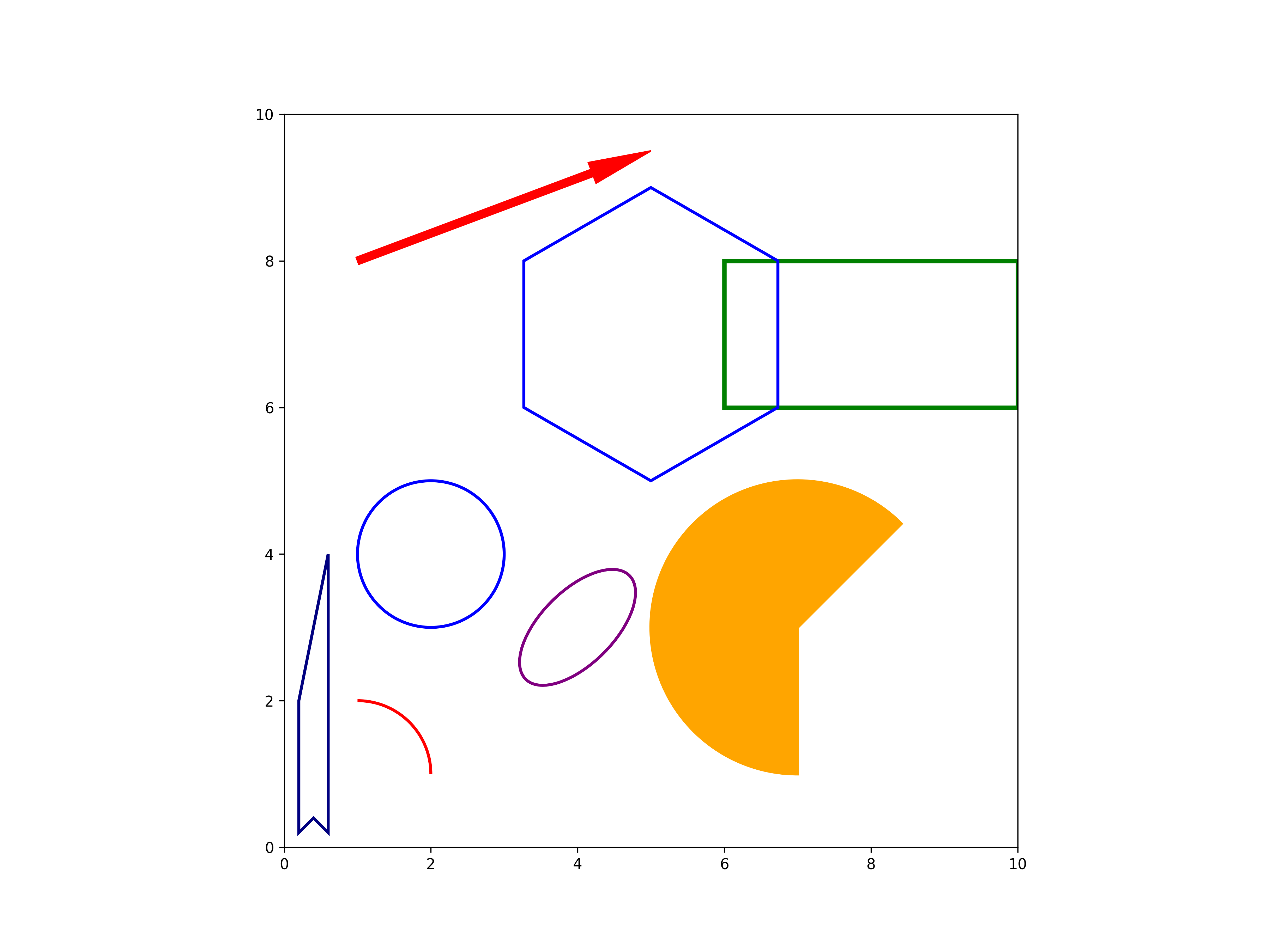
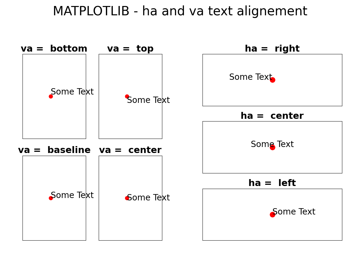
TEXT ALIGNMENT
When you add text to a plot, you specify its position using coordinates. You can adjust how the text aligns both vertically and horizontally with respect to this point bu using the va (vertical alignment) and ha (horizontal alignment) parameters.
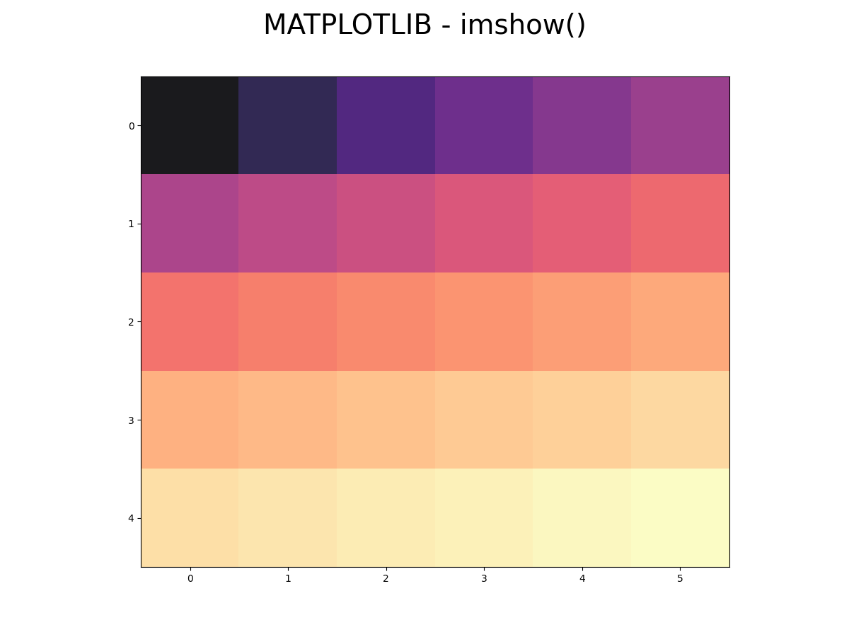
IMSHOW
The imshow() function is used to display an image or a sequence of number as an image
import matplotlib.pyplot as plt
import numpy as np
fig = plt.figure()
arr = np.linspace(1,10,30)
arr1=arr.reshape(5,6)
plt.imshow(arr2, cmap = 'magma', norm='log', alpha = 0.5)
plt.show()
QUIVER, CONTOUR, CONTOURF
The quiver function is used to plot 2D or 3D vectors with arrows, typically representing vector fields or directions. The example below illustrates how to create the directions of a 3D Cartesian coordinate system
import matplotlib.pyplot as plt
from mpl_toolkits.mplot3d import Axes3D
fig = plt.figure()
ax = fig.add_subplot(111, projection='3d')
ax.set_box_aspect([1, 1, 1],zoom=3)
ax.set_xlim(-1.5,1.5)
ax.set_ylim(-1.5,1.5)
ax.set_zlim(-1,1.5)
ax.set_axis_off()
ax.quiver(0,0,0, 1, 0, 0, color='blue', arrow_length_ratio=0.1)
ax.quiver(0,0,0, 0, 1, 0, color='blue', arrow_length_ratio=0.1)
ax.quiver(0,0,0, 0, 0, 1, color='blue',  arrow_length_ratio=0.1)
ax.text(1,0,-0.1,'x',color='black')
ax.text(0,1,0.1,'y',color='black')
ax.text(0,0.1,1,'z',color='black')
plt.show()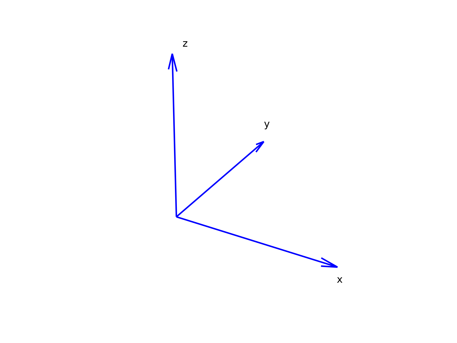
the scale argument can be used to adjust the size of the arrows in the plot
ax.quiver(X,Y,U,V,scale = 6,color='blue')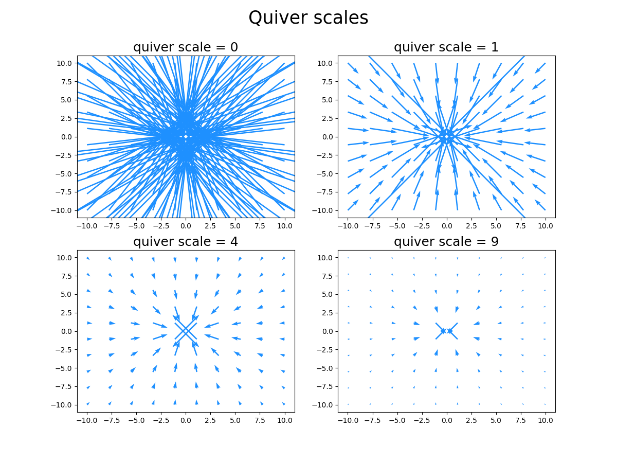
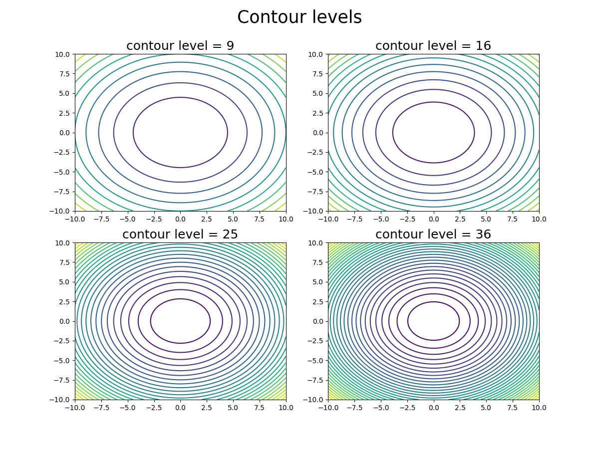
contour function is used to visualize and represent three-dimensional data by plotting contours, which are lines or surfaces connecting points of equal value in a two-dimensional plan
fig,axs = plt.subplots(2,2,figsize=(12,9))
fig.suptitle('Contour levels',fontsize=25)
x = np.linspace(-10,10,100)
y = np.linspace(-10,10,100)
X,Y = np.meshgrid(x,y)
Z = X**2+Y**2
n = len(axs.flatten())
levels = [ (x+3)**2 for x in range(n+1)]
for level, ax in zip(levels,axs.flatten()) :
    ax.set_title(f'contour level = {level}',fontsize=18)
    ax.contour(X,Y,Z,levels =level                    )
plt.show()
contourf
fig,axs = plt.subplots(2,2,figsize=(12,9))
fig.suptitle('Contourf levels',fontsize=25)
x = np.linspace(-10,10,100)
y = np.linspace(-10,10,100)
X,Y = np.meshgrid(x,y)
Z = X**2+Y**2
n = len(axs.flatten())
levels = [ (x+3)**2 for x in range(n+1)]
for level, ax in zip(levels,axs.flatten()) :
    ax.set_title(f'contourf levels = {level}',fontsize=18)
    ax.contourf(X,Y,Z,levels =level, cmap='viridis')
plt.show()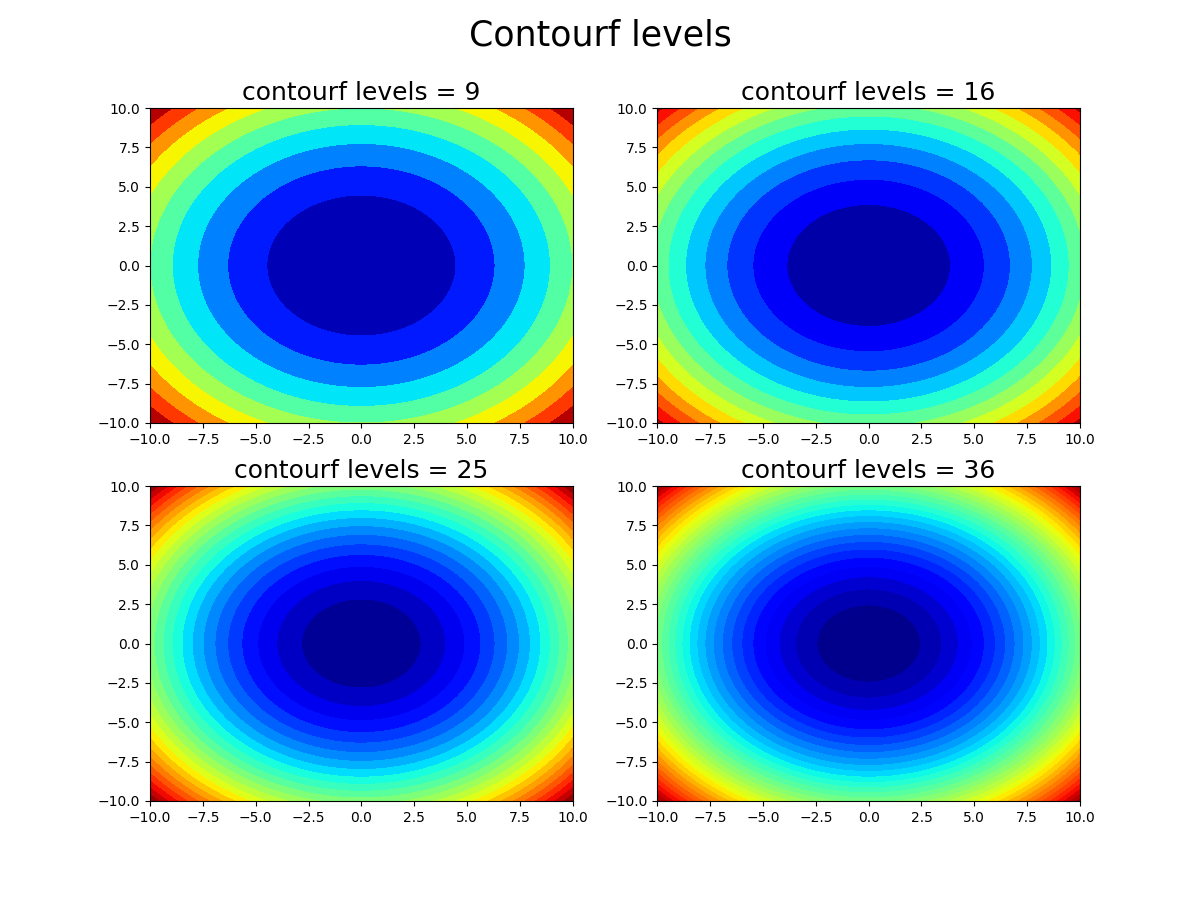
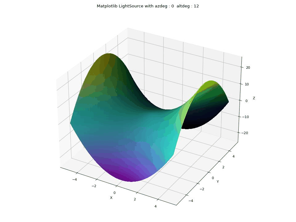
LIGHTSOURCE
The LightSource feature in Matplotlib is used to control the lighting and shading effects on a 3D surface plot. Azimuth and Altitude Control: allows you to set the azimuth (azdeg, 0-360 degrees clockwise) and altitude (altdeg, 0-90 degrees up from horizontal) angles, which determine the direction from which the virtual light source illuminates the surface.
from mpl_toolkits.mplot3d import Axes3D
from matplotlib.colors import LightSource
from matplotlib import cbook, cm
from matplotlib import pyplot as plt
import numpy as np
x = np.linspace(-5, 5, 300)
y = np.linspace(-5, 5, 300)
X, Y = np.meshgrid(x, y)
Z = X**2 - Y**2
fig,ax = plt.subplots(subplot_kw={'projection': '3d'})
ls = LightSource(azdeg=10, altdeg=30)
rgb = ls.shade(Z,cmap=cm.viridis, fraction=0.8, vert_exag=1)
ax.plot_surface(X, Y, Z, rstride=1,
                    cstride=1, linewidth=0, antialiased=False, facecolors=rgb)
plt.show()
This GIF illustrates the impact of changing the parameters of the LightSource feature in Matplotlib in Python on a 3D saddle-like surface. The parameters in focus are azdeg and altdeg, which determine the direction of the light source
SUBMODULES, TOOLKITS
Some submodules and toolkits of Matplotlib
from mpl_toolkits.mplot3d import Axes3D
from mpl_toolkits.mplot3d.art3d import Poly3DCollection
from matplotlib.colors import LightSource
from matplotlib import cbook, cm
import matplotlib.image as mpimg
from matplotlib.patches import Circle, Rectangle, Ellipse
import matplotlib.font_manager
from matplotlib import colors as mcolors
from matplotlib.colors import LightSource
SHAPES ON FIGURE
it's possible to draw shapes on the figure without worrying about the axes.
import matplotlib.pyplot as plt
import matplotlib.lines as lines
fig,ax = plt.subplots(2,2)
fig.add_artist(lines.Line2D([0,1],[1,0],color='green',linewidth=8))
fig.add_artist(lines.Line2D([0,1],[0,1],color='red',linewidth=8))
plt.show()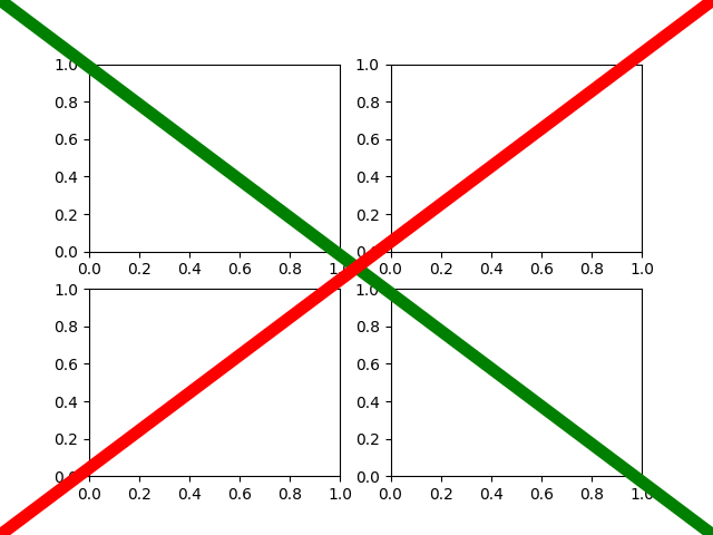
CHANGING SETTINGS WITH RCPARAMS
rcParams is a convenient tool when one wants to apply the same settings to all figures or axes. It provides a dictionary-like interface to set default values for various plot parameters.
mpl.rcParams refers to the global configuration and plt.rcParams to the current plot
rcParams : hide
import matplotlib as mpl
mpl.rcParams['axes.spines.top'] = False
mpl.rcParams['axes.spines.right'] = False
mpl.rcParams['axes.spines.bottom'] = False
mpl.rcParams['axes.spines.left'] = False
mpl.rcParams['xtick.bottom'] = False
mpl.rcParams['ytick.left'] = False
mpl.rcParams['xtick.labelbottom'] = False
mpl.rcParams['ytick.labelleft'] = False
# 3D :
mpl.rcParams['axes3d.xpane.fill'] = False
mpl.rcParams['axes3d.ypane.fill'] = False
mpl.rcParams['axes3d.zpane.fill'] = False
rcParams : more on ticks, ticks labels and spines
plt.rcParams['xtick.color'] = 'blue'
plt.rcParams['ytick.color'] = 'purple'
plt.rcParams['xtick.labelsize'] = 12
plt.rcParams['ytick.labelsize'] = 12
rcParams : fonts
plt.rcParams['font.family'] = 'serif'
plt.rcParams['text.color'] = 'cyan'
rcParams : LaTex
plt.rcParams['text.usetex'] = True
plt.rcParams['text.latex.preamble'] = r'\usepackage{amsmath}'