NUMPY

---

Skip to a subsection :

1. WHAT'S NUMPY ?
2. ARRAYS
3. CREATING ARRAYS
4. PROPERTIES OF ARRAYS
5. SLICING, INDEXING
6. ACCESS METHODS
7. APPEND, CONCATENATE, REMOVE
8. OPERATIONS
9. MATHEMATICAL FUNCTIONS
10. LINEAR ALGEBRA
11. LOOPING OVER AN ARRAY

---

1. WHAT'S NUMPY

NumPy is a large and powerful library for numerical computing Python, and it provides a wide range of functions for working with large, multi-dimensional arrays and matrices. While it is certainly useful to learn as many of these functions and data structures as possible, it is not necessary to learn all of them in order to begin working with data in Python. Instead, it is often sufficient to start with the most important and commonly used functions, and then gradually learn more advanced features as you need them. This can help you get started more quickly and avoid getting overwhelmed by the wealth of features available in the library. By learning these and other basic functions and data structures in NumPy, you will be well-equipped to start working with data in Python and perform a wide range of data analysis tasks. As you continue to learn and grow as a data analyst, you can gradually learn more advanced features of the library as needed. The exact number of functions available in NumPy can vary depending on the version of the library you are using, but there are over 1000 functions available.

2. ARRAYS

In programming, an array is a data structure that stores a collection of elements of the same data type. It's similar to a list, but with a key difference: arrays have a fixed size, which means that you can't add or remove elements from them once they're created.NumPy arrays are more powerful than Python's built-in lists because they allow you to perform mathematical operations on entire arrays at once, rather than having to loop through each element. This makes NumPy arrays much faster and more efficient for numerical computations. NumPy arrays can have any number of dimensions, from 0 (a scalar value) to n (a multidimensional array). Each element in a NumPy array must be of the same data type, which is typically either integers or floating-point numbers

The shape of an array refers to its dimensions or the size of each dimension. A 1D array has a single dimension, and its shape is given by the number of elements it contains. A 2D array, on the other hand, has two dimensions and its shape is given by the number of rows and columns. The shape argument is often used in methods that create new arrays. It takes a tuple as its value, where each element of the tuple represents the size of a dimension in the new array. For example, if you want to create a 2D array with 3 rows and 4 columns, the shape argument is a tuple (3, 4). If you want to create a 1D array with 5 elements, the shape argument is a tuple (5,)

An array of dimension 1 and shape (3,)  :
[4, 2, 3]

An array of dimension 2 and shape (2,3) :
[[4, 2, 3],
 [1, 1, 5]]

An array of dimension 3 and shape (2,3,2) :
[[[1, 3], [4, 1], [1, 1]],
 [[2, 3], [4, 4], [0, 2]]]

3. CREATING ARRAYS

SPECIFYING ALL VALUES

This method of array creation is commonly used when you want to create a NumPy array with a small number of known values.

import numpy as np
# Creating a 1D array
arr=np.array([1,3,5,7])
print(arr) # prints [1 3 5 7]

# Creating a 2D array
arr=np.array([[1,3,5,7],[2,4,6,8]])
print(arr) # prints [[1 3 5 7] [2 4 6 8]]

# Creating a 3D array
arr=np.array([[[1,2,3],[4,5,6]],[[0,0,0],[1,1,1]]])
print(arr) # prints [[[1 2 3] [4 5 6]] [[0 0 0] [1 1 1]]]

from LIST

If you're already familiar with using variables, you can start working with NumPy arrays by creating an array from a list that you've stored in a variable. This is a useful way to get started with NumPy, because it allows you to use your existing knowledge to create and manipulate arrays.

import numpy as np
mylist=[1,3,5,7]
arr=np.array(mylist)
print(arr) # prints [1 3 5 7]
print(type(arr)) # prints numpy.ndarray

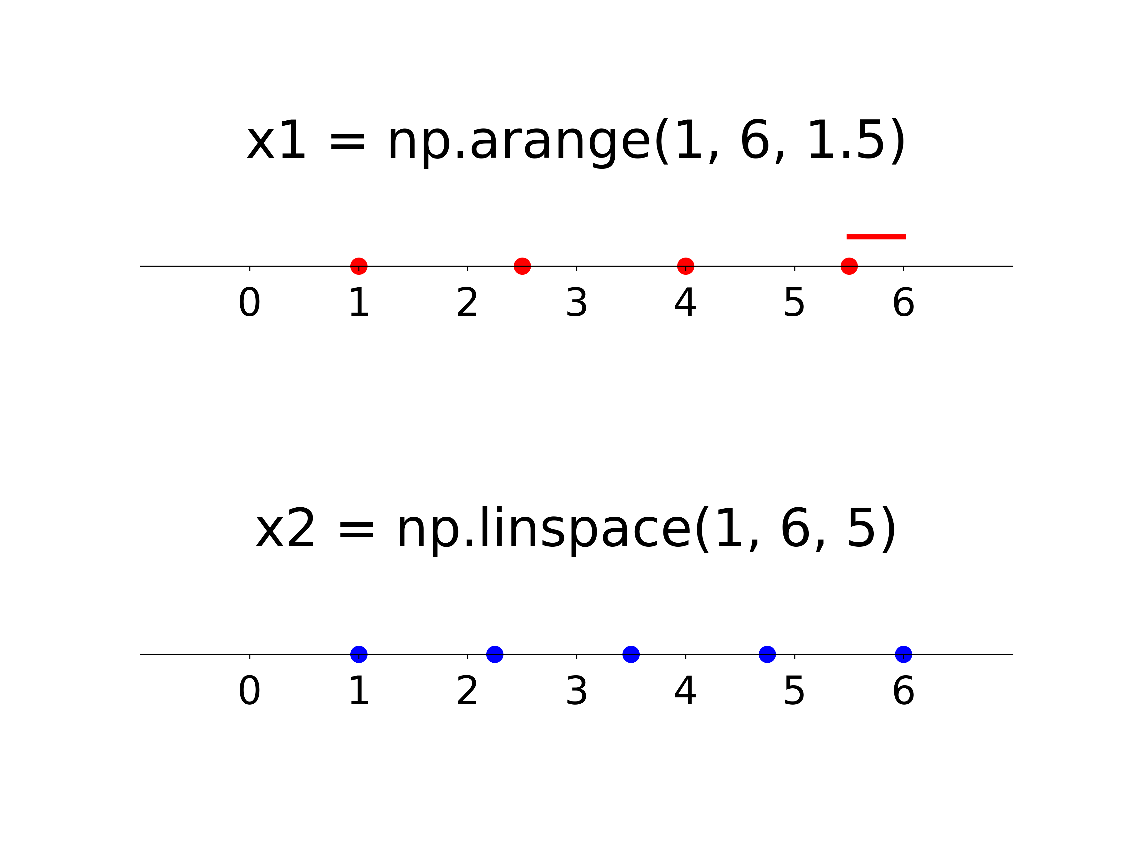
ARANGE

arange is used to create an array of equally spaced values with a specified step within a given range. It takes three arguments: start, stop, and step.

import numpy as np
# Creating a 1D array with arange() : 
arr=np.arange(0,12,2)
print(arr) # prints [ 0  2  4  6  8 10]

# Creating a 2D array with arange() and reshape() :
arr=np.arange(0,12,2).reshape((2,3))
print(arr) # prints [[ 0  2  4] [ 6  8 10]]

LINSPACE

linspace is used to create an array of evenly spaced values with a specified number of elements within a given interval.. It takes three arguments: start, stop, and num.

import numpy as np
arr=np.linspace(0,12,3)
print(arr) # prints [ 0.  6. 12.]

RANDOM

random.randint() is a function that generates random integers within a specified range. It takes three arguments: low, high, and size. Size is an optional argument that specifies the shape of the output array.

import numpy as np
arr=np.random.randint(0, 10, size = (2,2))
print(arr) # prints [[3 4] [3 0]]     

random.rand() is a function that generates random numbers from interval [0,1]. The lower boundary (0) is inclusive. The upper boundary (1) is exclusive.

import numpy as np
arr=np.random.rand(1,4)
print(arr) # prints [[0.16996073, 0.49633693, 0.34702019]]

random.permutation() is a function that randomly shuffles an array. It takes one argument: x, which is the input array

import numpy as np
arr=np.array([1,2,3,4])
arr2=np.random.permutation(arr)
print(arr2) # prints [2 3 4 1]

arr=np.random.permutation(5)
print(arr) # prints [0 1 3 4 2]

random.choice() is a function that randomly select elements from a NumPy array. You can select a single element or several elements, with or without replacement.

import numpy as np
arr=np.array([1,2,3])

element=np.random.choice(arr)
print(element) # prints 3

elements=np.random.choice(arr,2,replace=True)
print(elements) # prints [3,3]

elements=np.random.choice(arr,2,replace=False)
print(elements) # prints [1,3]

RANDOM DISTRIBUTIONS

NumPy can generate arrays of random numbers using probabilistic distributions like Gaussian (normal) distributions and Poisson distributions.

import numpy as np

# Uniform distribution
np.random.uniform(low=1,high=10,size=15)

# Normal (Gaussian) Distribution, with loc=mean and scale=std_dev
np.random.normal(loc = 10,scale=2,size = 15)

# Exponential Distribution
np.random.exponential(scale = 2, size = 15)

# Gamma Distribution
np.random.gamma(shape = 2, scale = 3, size = 15)

# Poisson Distribution:
np.random.poisson(lam = 3.5, size = 15)

# Binomial Distribution with n = number of trials and p = probability of succes :
np.random.binomial(n = 10, p = 0.3, size = 15)

# Geometric Distribution, with p = probability of succes
np.random.geometric(p = 0.3, size = 15)

# Bivariate Gaussian Distribution
n_samples = 500
mean_height = 165
std_height = 10
mean_weight = 70
std_weight = 8
correlation = 0.7
cov_matrix = np.array([[std_height**2, correlation * std_height * std_weight],
                       [correlation * std_height * std_weight, std_weight**2]])
np.random.multivariate_normal([mean_height, mean_weight], cov_matrix, n_samples)

EMPTY

empty() creates a new empty array , it allocates a block of memory for the array but doesn't initialize its values. This means that the contents of the array are undefined, and could contain any values that happen to be in memory at the time the array is created.

import numpy as np
arr=np.empty((3,))
print(arr) # prints any values that happen to be in memory at the time the array is created    

ZEROS

np.zeros() creates a new array of a specified shape and data type, filled with zeros. It takes one argument: shape, which is a tuple that specifies the dimensions of the array.

import numpy as np
# Creating a 1D array with .zeros()
arr=np.zeros((3,))
print(arr) # prints [0. 0. 0.]

# Creating a 2D array with .zeros()
arr=np.zeros((3,2))
print(arr) # prints [[0. 0.] [0. 0.] [0. 0.]]

ONES

ones() creates a new array of a specified shape and data type, filled with zeros. It takes one argument: shape, which is a tuple that specifies the dimensions of the array.

import numpy as np
# Creating a 1D array with .ones()
arr=np.ones((3,))
print(arr) # prints [1. 1. 1.]

# Creating a 2D array with .ones()
arr2=np.ones((3,2))
print(arr2) # prints [[1. 1.] [1. 1.] [1. 1.]]

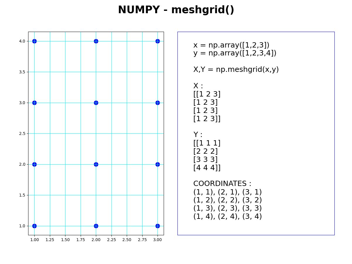
MESHGRID

meshgrid() is used to create a grid of coordinates from two or more arrays of coordinate values. It returns 2 arrays with the same shape which can be used to compute the value of a function at each point of the grid

import numpy as np
x = np.array([0,1,2])
y = np.array([0,1,2])
X, Y = np.meshgrid(x, y)   
print(X) # prints [[0 1 2][0 1 2][0 1 2]]
print(Y) # prints [[0 0 0][1 1 1][2 2 2]]

from NPY or NPZ FILE

load() function opens a NumPy array from a .npy .npz file. The extension for a NumPy array saved as a single array file is .npy, while the extension for a NumPy array saved as a compressed archive of multiple arrays is .npz. load() returns a numpy array which you can assign to a variable. In the cases below, an array is saved as a single array file .npy and two arrays are saved as a compressed archive file .npz . Then the saved data is loaded using load() and stored in variables

import numpy as np
arr1 = np.array([1, 2, 3])
arr2 = np.array([4, 5, 6])
np.save('my_array.npy', arr1)
arr = np.load('my_array.npy')

np.savez('my_arrays.npz', arr1=arr1, arr2=arr2)
data = np.load('my_data.npz')
arr1 = data['arr1']

from IMAGE

If you are familiar with the Python imaging library Pillow, you can load an image and store it as a NumPy array using just a few lines of code and the asarray() function.

from PIL import Image
import numpy as np
image = Image.open('my_image.jpg')
array = np.asarray(image)

from TXT FILE

genfromtxt() loads an array from a text file. By default, genfromtxt() will try to automatically detect the format of the data in the file and load it into a NumPy array. You can specify additional arguments to control how the data is loaded

import numpy as np
data = np.genfromtxt('mydata.txt')
data = np.genfromtxt('mydata.txt', delimiter=',')
data = np.genfromtxt('mydata.txt', skip_header=1)

4. PROPERTIES OF ARRAYS

Here a some common numpy array properties. As they are properties of an array object, rather than methods, they are accessed using dot notation after an array object, such as arr.shape or arr.ndim, where arr is the name of the array. Unlike methods, which are called using parentheses after their name, properties are accessed without parentheses.

shape : returns a tuple that specifies the size of each axis, or dimension, of the array.

dtype: type of data stored in the array ( integers, floats ...)

size : returns the type of data stored in the array

ndim : returns the number of dimensions of the array

arr=np.array([[4,2,3],[1,1,5]])
print(arr.shape) # prints (2, 3)
print(arr.dtype) # prints dtype('int32')
print(arr.size) # prints 6
print(arr.ndim) # prints 2

5. SLICING, INDEXING

Slicing allows you to extract a portion of an array by specifying a range of indices. The square brackets [] are used to index and slice both lists and numpy arrays. You can extract individual elements or slices of elements.

• The index of the first element is zero, not one
• Slicing is inclusive of the element at the start index
• Slicing is exclusive of the element at the stop index
• To access elements of a multi-dimensional array, you can use multiple sets of square brackets [].

Slicing a 1D array :

arr=np.array([4,1,5])

# get the first element of the array arr:
print(arr[0]) # prints 4

# get an array that contains a slice of array arr
print(arr[0:1]) # prints [4]
print(arr[0:2]) # prints [4 1]

    

Slicing a 2D array :

arr=np.array([[4,2,3],[1,1,5],[0,9,7]])

# get the first element of the array arr:
print(arr[0]) # prints [4 2 3]

# get the first element of the second element of array arr:
print(arr[1][0]) # prints 1

# get a slice of 2 elements of array arr :
print(arr[1:3]) # prints [[1 1 5] [0 9 7]]
        

Boolean indexing :

arr=np.array([4,1,5])
arr2=arr[arr>1]
print(arr2) # prints array([4, 5])

6. ACCESS METHODS

np.take() function allows you to retrieve elements using a list of indices

arr = np.array([1,2,3,4,5])
arr2 = np.take(arr,[0,4])
print(arr2) # prints array([1, 5])

np.nonzero() is function returns the indices of elements that are non-zero in an array

arr = np.array([1,0,3,0,5])
arr2=np.nonzero(arr)
print arr2 # prints array([0, 2, 4])

ndarray.flat() provides a 1-dimensional iterator over the array elements. It allows you to access each element of the array one by one

np.ravel() or ndarray.flatten() are functions that flatten a multi-dimensional array into a 1-dimensional array.

7. APPEND, CONCATENATE, REMOVE

The numpy.append() function is used to append a new element to an existing my_array.

my_array = np.array([1, 2, 3])
new_element = 4
new_array = np.append(my_array, new_element)
print(new_array) # [1 2 3 4]    

The numpy.delete() function is used to remove elements from an array

my_array = np.array([1, 2, 3, 4])    
new_array = np.delete(my_array, 2)
print(new_array) # prints [1 2 4]

you can also use boolean indexing to remove some elements :

arr = np.array([1, 2, 3, 4])    
new_array = arr[arr !=3]
print(new_array) # prints [1 2 4]

np.hstack() is used to horizontally stack arrays. It concatenates arrays along their horizontal axis. np.vstack() is used to verticalally stack arrays. It concatenates arrays along their vertical axis

arr1 = np.array([[1, 2], [3, 4]])
arr2 = np.array([[5, 6], [7, 8]])
stacked_array_h = np.hstack((arr1, arr2))
print(stacked_array_h) # prints array([[1, 2, 5, 6], [3, 4, 7, 8]])
stacked_array_v = np.vstack((arr1, arr2))
print(stacked_array_v) # prints array([[1, 2], [3, 4], [5, 6], [7, 8]])

np.insert() is used to insert values along a specified axis:

arr = np.array([[1, 2], [3, 4]])
new_arr = np.insert(arr, 1, [8, 9], axis=1)
print(new_arr) # prints array([[1, 8, 2], [3, 9, 4]]) 
new_arr = np.insert(arr, 1, [8, 9], axis=0)
print(new_arr) # prints array([[1, 2], [8, 9], [3, 4]])

8. OPERATIONS

Addition of two arrays is performed element-wise. This means that each element in the first array is added to the corresponding element in the second array, resulting in a new array of the same shape as the original arrays. Similarly, subtraction, multiplication, and division are also performed element-wise.

When using the * operator with NumPy arrays, it performs element-wise multiplication between arrays of the same shape. On the other hand, matrix multiplication between arrays is done using the @ operator or the dot() method.

Here is a list of element-wise operations :

• Addition (+)
• Subtraction (-)
• Multiplication (*)
• Division (/)
• Integer division (//)
• Modulus (%)
• Exponentiation (**)
• Absolute value (abs())
• Trigonometric functions (np.sin(), np.cos(), etc.)
• Logarithmic functions (np.log(), np.log10(), etc.)
• Comparison operators (>, <, ==, !=, etc.)

np.vectorize() : if you want to apply a custom function to each element of a NumPy array. This is where np.vectorize could come in handy. However, this may be less efficient compared to directly using the element-wise functions provided by NumPy as mentioned earlier

import numpy as np
a = np.array([-1, 2, -3, 4])
def f(x):
    if x < 0:
        return np.sin(x)
    else:
        return x ** 2
vectorized_function = np.vectorize(f)
result = vectorized_function(a)
print(result)
# prints : [-0.84147098  4.  -0.14112001 16. ]

9. MATHEMATICAL FUNCTIONS

In addition to working with numpy arrays, some of these functions can also be used on other objects, such as integers or floating-point numbers. This can be very convenient, as it eliminates the need to import additional modules or libraries to perform certain mathematical operations. For example, numpy provides a function called numpy.pi, which returns the value of pi to a specified precision. This function can be used like any other numpy function, even though it is not operating on a numpy array. Another example is the numpy.power function, which raises a number to a specified power. This function can be used with any numerical object, such as an integer or a floating-point number

np.round(): to round the values of a NumPy array to the nearest value. It takes an array (or a single number) with decimal values as input and returns an array with those values rounded to the specified number of decimal places.

import numpy as np
    arr = np.array([[65.91, 170.7], [70.12, 175.299]])
    arr = np.round(arr,1)

np.sign() : returns the sign of each element : -1 for negative elements, 0 for zero, and 1 for positive elements.

import numpy as np
arr = np.array([-1, 2, -3, -4])
print(np.sign(arr)) # prints [-1  1 -1 -1]

np.roots : to get the roots of a polynomial

import numpy as np
p1 = np.array([1,-4,2])
print(np.roots(p1)) # prints [3.41421356 0.58578644]
p2 = np.array([2,-1,2])
print(np.roots(p2)) # prints [0.25+0.96824584j 0.25-0.96824584j]

np.polyval : to calculate the value of a polynomial function for a given value of the variable

import numpy as np
x0 = 0
x1 = np.linspace(-10,10,5)
# coefficients in descending order of degree
coefficients = [2, -3, 1]
y0 = np.polyval(coefficients, x0)
y1 = np.polyval(coefficients, x1)
print(y0) # prints 1
print(y1) # prints [231.  66.   1.  36. 171.]

NumPy provides a set of statistical functions for analyzing and manipulating numerical data :

• np.sum()
• np.mean()
• np.median()
• np.var()
• np.std()
• np.min()
• np.max()
• np.percentile()
• np.histogram()
• np.cov()
• np.corrcoef()
• np.unique()

np.corrcoef(): to calculate the correlation matrix for variables. The rowvar=False argument indicates that each column represents a variable

import numpy as np
dataset = np.array([[65, 170], [70, 175], [63, 165], [75, 180], [68, 172]])
correlation_matrix = np.corrcoef(dataset, rowvar=False)

complex numbersNumpy allows to use a complex number class, and you can do it like this :

import numpy as np
z = 1 + 2j
print(z) # prints (1+2j)
print(type(z)) # prints 'complex'
print(np.real(z)) # prints 1.0
print(np.imag(z)) # prints 2.0
print(np.conj(z)) # prints (1-2j)
print(np.exp(1j*np.pi/3)) # prints (0.5000000000000001+0.8660254037844386j)
argument = np.angle(1j)
modulus = np.abs(1+2j)
a,b = 1,2
z = a + b*1j
print(z) # prints (1+2j)

10. LINEAR ALGEBRA

Numpy provides several functions for linear algebra, which makes it useful for working with vectors and matrices. They are represented as arrays. In mathematics, vectors are typically represented as column vectors, which are vertical arrays with a single column. However, in NumPy, vectors are often represented as one-dimensional arrays.

import numpy as np

# dot product of 2 vectors
v1=np.array([1,1])
v2=np.array([-1,1])
print(np.dot(v1,v2)) # prints 0

# cross product of 2 vectors
v1=np.array([2,0,0])
v2=np.array([0,3,0])
print(np.cross(v1,v2)) # prints [0 0 6]

# outer product of 2 vectors
v1=np.array([2,3])
v2=np.array([-5,7])
print(np.outer(v1,v2)) # prints [[-10  14] [-15  21]]

# norm of a vector
v3=np.array([3,4])
print(np.linalg.norm(v3)) # prints 5.0

# distance between 2 points A and B
a = np.array([3, 1])
b = np.array([3, 2])
distance = np.linalg.norm(b - a)
print(distance) # prints 1.0
print(type(distance)) # prints numpy.float64


# identity array
identity_array = np.eye(3)

# triangular arrays
arr=np.ones((4,4))
arr_low=np.tril(arr)
arr_up=np.triu(arr)

# matrix product : matmul or @
v4 = np.array([[1, 2], [3, 4]])
v5= np.array([[5, 6], [7, 8]])
print(np.matmul(v4, v5)) # prints array([[19, 22], [43, 50]])
print(v4@v5) # prints array([[19, 22], [43, 50]])

# product of a rotation matrix and a vector
a=np.pi/2
v1=np.array([1,1])
arr=[[np.cos(a),-np.sin(a)],[np.sin(a),np.cos(a)]]
print(arr@v1) # prints array([-1.,  1.])

# determinant of a matrix A 
A = np.array([[2, 3], [4, 1]])  
det_A = np.linalg.det(A)  
print("Determinant of A:", det_A) # returns -10

# invert a matrix A 
A = np.array([[2, 1], [3, 4]])
inv = np.linalg.inv(A)
print(inv) # prints array([[ 0.8, -0.2],[-0.6,  0.4]])

# solve a Cramer's system of dimension 2 AX=B
A = np.array([[2, 3], [4, 1]])  # Coefficient matrix A
B = np.array([7, 5])  # Right-hand side vector B
X = np.linalg.solve(A, B)  # Solve the system
x = X[0]  # Solution for x
y = X[1]  # Solution for y
print(x)
print(y)

# eigenvalues , eigenvectors
m = np.random.randint(1,4,9).reshape(3,3)
print(np.linalg.eig(m)) # prints :
# EigResult(eigenvalues=array([ 5.        , -1.61803399,  0.61803399]), 
# eigenvectors=array([[-0.4738791 , -0.5       , -0.5       ],
#       [-0.65158377,  0.80901699, -0.30901699],
#       [-0.59234888, -0.30901699,  0.80901699]]))

11. LOOPING OVER AN ARRAY

There are multiple ways to iterate over an array :

import numpy as np
#  4 ways to access elements of a 2D NumPy array using a loop :
arr=np.array([[0, 1, 2],
    [3, 4, 5]])

# 1
for row in arr:
    for element in row :
        print(element)
# 2
for index, value in np.ndenumerate(arr):
    print(index, value)

# 3    
for i in range(arr.shape[0]):
    for j in range(arr.shape[1]):
        element = arr[i, j]
        print(element)

# 4 
for element in np.nditer(arr):
    print(element)
        
# 2 ways to modify elements of a 2D NumPy array using a loop :

# 1 
for i in range(len(arr)):
    for j in range(len(arr[i])):
        arr[i, j] = arr[i, j] ** 2
print(arr)

# 2
for index, value in np.ndenumerate(arr):
    arr[index] = value ** 2
print(arr)