REGRESSION MODELS
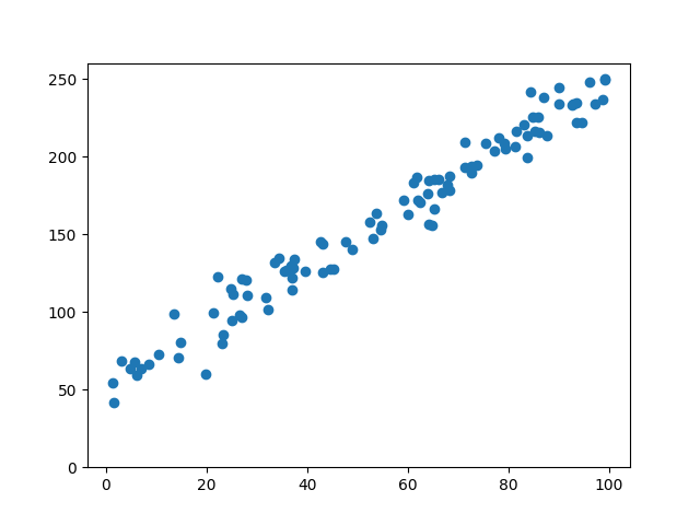
LINEAR REGRESSION
Python offers several options for performing linear regression.
First, let's create a simple dataset of real variables. The variable y depends on x linearly, and we add some noise to make it more realistic
import numpy as np
def f1(x, slope = 1, intercept = 0):
    return slope * x + intercept
vect_f1 = np.vectorize(f1)
x = np.random.uniform(low = 1, high = 100, size = 100)
noise = np.random.normal(loc = 0, scale = 10, size = 100)
y = vect_f1(x,2,50) + noise
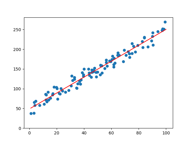
Python provides librairies to calculate the properties of a linear regression line, but you can also create custom functions based on statistical formulas to achieve the same results. While this approach may be more time-consuming, it can provide a clearer understanding of the underlying calculations
Calculating Linear Regression Manually :
def linear_regression_line(x,y):
    slope = (np.sum(( x - np.mean(x)) * (y - np.mean(y)))) / np.sum((x - np.mean(x)) ** 2 )
    intercept = np.mean(y) - slope * np.mean(x)
    return slope, intercept
slope, intercept = linear_regression_line(x,y)
Calculating Linear Regression using scikit-learn :
from sklearn.linear_model import LinearRegression
model = LinearRegression()
model.fit(x.reshape(-1, 1), y)  # Reshape x (1D to 2D column)
slope = model.coef_[0]
intercept = model.intercept_
Calculating Linear Regression using scipy :
from scipy.stats import linregress
slope, intercept, r_value, p_value, std_err = linregress(x, y)
All the above-mentioned approaches will return the same slope and intercept.
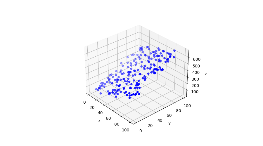
MULTIPLE LINEAR REGRESSION
Just as with simpel linear regressions, there are several options available.
let's create a multiple linear dataset of real variables and add some noise
def g(x,y):
    z = 3 * x + 4 * y + 5
    return z
vect_g1 = np.vectorize(g)
x = np.random.uniform(low = 1, high = 100, size = 200)
y = np.random.uniform(low = 1, high = 100, size = 200)
noise = np.random.normal(loc = 0, scale = 10, size = 200)
z = vect_g1(x,y) + noise
Calculating Multiple Linear Regression using Numpy :
# Organize the data into a matrix X by stacking x and y
X = np.vstack((x, y)).T
# Add a bias (constant) column to X
X = np.column_stack((X, np.ones_like(x)))
# Use the NumPy linear regression function to fit the model
coefficients = np.linalg.lstsq(X, z, rcond=None)[0]
# The coefficients are in the order a, b, c with z = a * x + b * y + c
a, b, c = coefficients
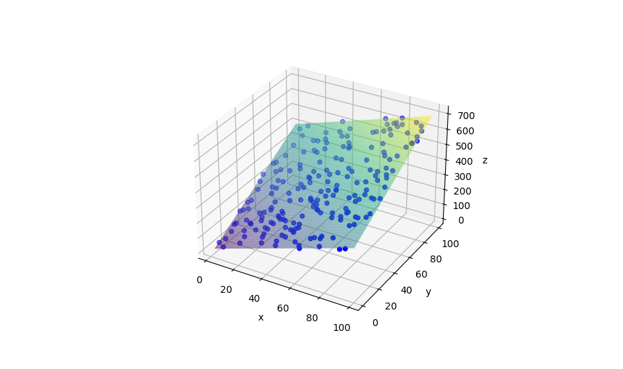
Plotting data and regression plan
fig,ax = plt.subplots(figsize=(12,9), subplot_kw={'projection': '3d'})
ax.scatter(x, y, z, c='b')
ax.set_xlabel('x')
ax.set_ylabel('y')
ax.set_zlabel('z')
x_grid, y_grid = np.meshgrid(np.linspace(min(x), max(x), 100), np.linspace(min(x), max(y), 100))
z = a * x_grid + b * y_grid + c
ax.plot_surface(x_grid, y_grid, z, alpha=0.5, cmap='viridis', label='Regression Plane')
plt.show()
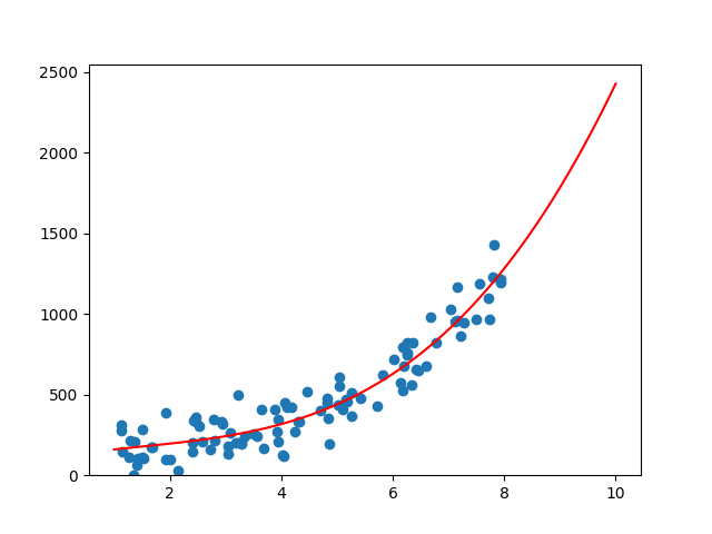
POLYNOMIAL REGRESSION
Just as with linear regressions, there are several options available. Let's find the coefficients of a polynomial regression using a manual approach before using libraries
let's create a simple a non linear dataset of real variables and add some noise
def f2(x):
    return 2*x**3 + 200
vect_f2 = np.vectorize(f2)
x = np.random.uniform(low = 1, high = 8, size = 100)
noise = np.random.normal(loc = 0, scale = 100, size = 100)
y = vect_f2(x) + noise
Calculating Polynomial Regression Manually :
X_mat=np.vstack([np.ones_like(x), x, x**2, x**3]).T
# ascending order of degree
    coefficients_manual = np.dot(np.dot(np.linalg.inv(np.dot(X_mat.T,X_mat)),X_mat.T),y)
Calculating Polynomial Regression using Numpy :
# descending order of degree
coefficients_np = np.polyfit(x, y, 3)
Calculating Polynomial Regression using scikit-learn :
from sklearn.linear_model import LinearRegression
    from sklearn.preprocessing import PolynomialFeatures
    poly = PolynomialFeatures(degree = 3)
    X_poly = poly.fit_transform(x.reshape(-1, 1))
    model = LinearRegression().fit(X_poly, y)
    # ascending order of degree :
    coefficients_sk = model.coef_ # coefficients without degree 0
    intercept = model.intercept_ # degree 0
All the above-mentioned approaches will return the same coefficients, although the order in which the coefficients are presented may vary depending on the methods used.
- scikit-learn : ascending order of degree
- numpy : descending order of degree
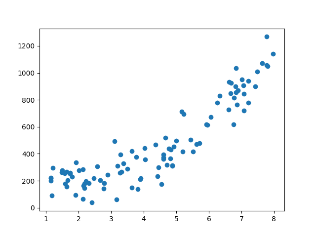
Plotting data and polynomial values
fig , ax = plt.subplots()
x_reg = np.linspace(1,10,100)
y_reg = np.polyval(coefficients_np, x_reg)
plt.scatter(x,y)
plt.plot(x_reg,y_reg,'red')
ax.set_ylim(bottom = 0)
plt.show()