PythonKeys

Skip to a subsection :

3D projection
subplots with 2D and 3D
SURFACES
LIGHTSOURCE
POLYGON 3D

3D PROJECTIONS

To represent a 3D object using Matplotlib, you need to start by selecting a 3D projection, and there are several ways to do this :

from matplotlib import pyplot as plt
from mpl_toolkits.mplot3d import Axes3D
ax = fig.add_subplot(111, projection='3d')
fig,ax = plt.subplots(subplot_kw={'projection': '3d'})
fig,axs = plt.subplots(3,4,subplot_kw={'projection': '3d'})

SUBPLOTS WITH BOTH 2D AND 3D

While it may not be very straightforward, it is possible to have both a 2D axis and a 3D axis coexist on the same figure. This example shows how to create a figure with both a 2D and a 3D plot, while utilizing the "mosaic" function to manage their proportions within the figure's width

from matplotlib import pyplot as plt
from mpl_toolkits.mplot3d import Axes3D
mos=[['A','A','A','B','B']]
fig, axs = plt.subplot_mosaic(mos,figsize=(12,9))
axs['A'].spines['top'].set_visible(False)
axs['A'].spines['right'].set_visible(False)
axs['A'].spines['bottom'].set_visible(False)
axs['A'].spines['left'].set_visible(False)
axs['A'].tick_params(axis='both', which='both', length=0, labelsize=0)
axs['A'].set_yticks([])
axs['A'] = fig.add_subplot(121,projection='3d')
x=np.linspace(-10,10,100)
y1=np.linspace(-10,10,100)
y2=np.exp(x)
z = x**2*np.sin(y1)
axs['A'].plot(x,y1,z,color='blue')
axs['B'].plot(x,y2,color='red')
plt.show()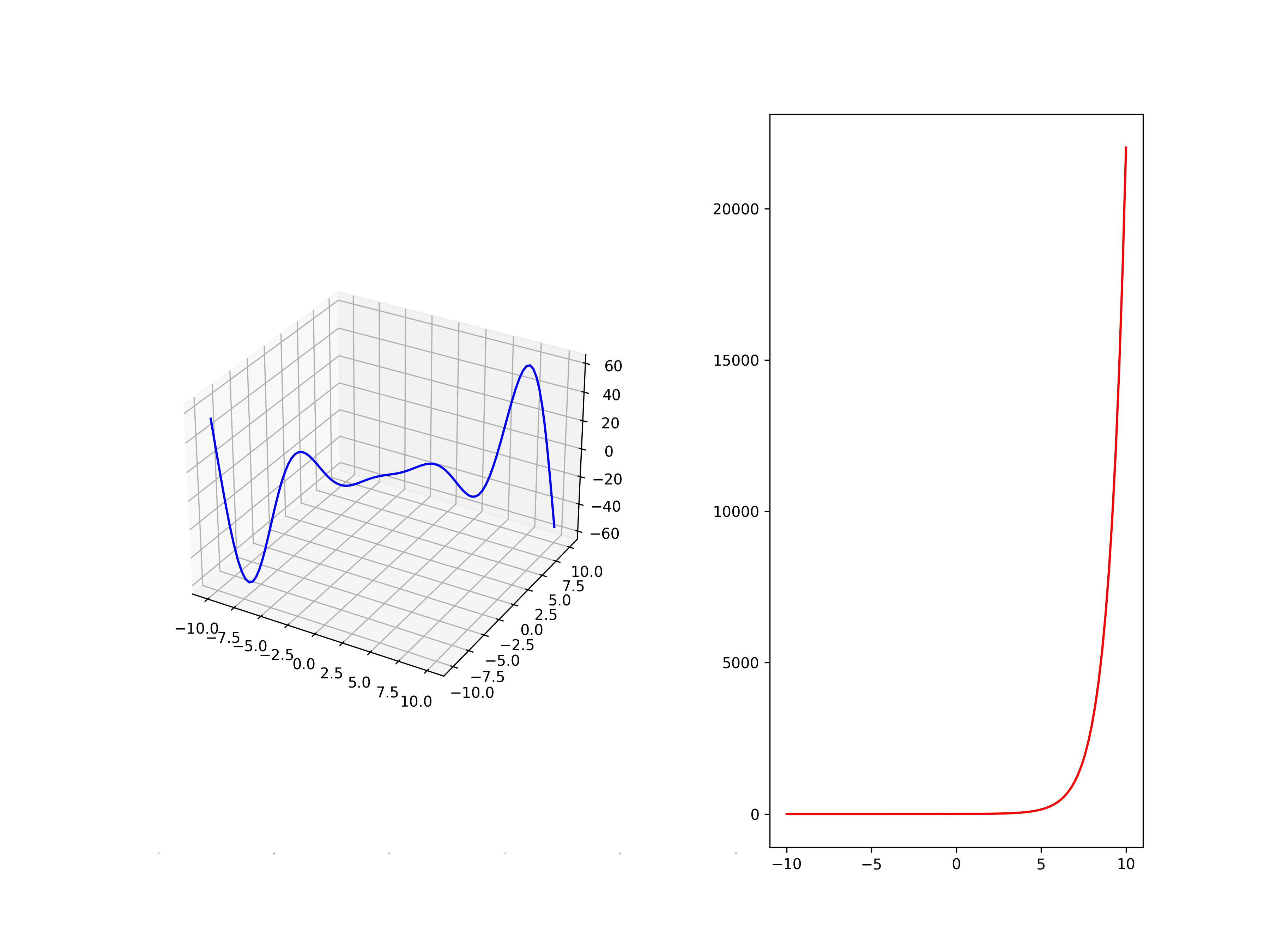

SURFACES

Plot a surface with meshgrid :

import matplotlib.pyplot as plt
import numpy as np
from mpl_toolkits.mplot3d import Axes3D    
def f(x, y):
    return np.sin(np.sqrt(x**2 + y**2))
x = np.linspace(-5, 5, 50)
y = np.linspace(-5, 5, 50)
X, Y = np.meshgrid(x, y)
Z = f(X, Y)
fig = plt.figure()
ax = fig.add_subplot(111, projection='3d')
ax.plot_surface(X, Y, Z, cmap='viridis')
ax.set_xlabel('X')
ax.set_ylabel('Y')
ax.set_zlabel('Z')
plt.show()

Plot a surface with trisurf :

triangulated surface.

import matplotlib.pyplot as plt
import numpy as np
from mpl_toolkits.mplot3d import Axes3D    
fig = plt.figure()
ax = fig.add_subplot(111, projection='3d')
x = [0,1,2,0]
y = [2,1,1,3]
z = [1,1,1,2]
ax.plot_trisurf(x,y,z,facecolor='red',alpha=0.2)
plt.show()

LIGHTSOURCE

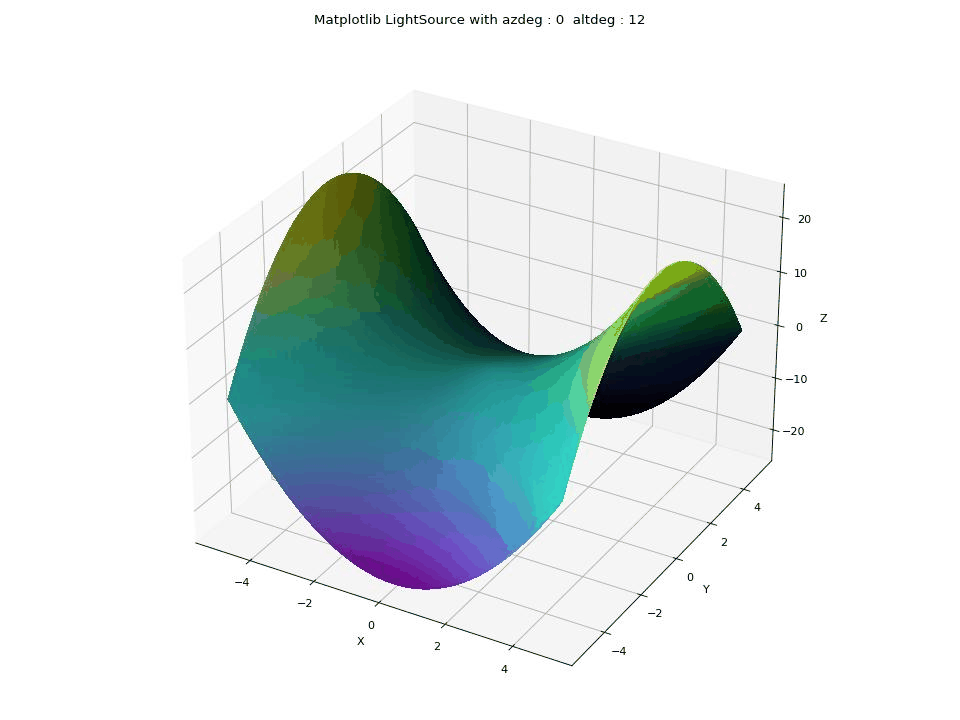
The LightSource feature in Matplotlib is used to control the lighting and shading effects on a 3D surface plot. Azimuth and Altitude Control: allows you to set the azimuth (azdeg, 0-360 degrees clockwise) and altitude (altdeg, 0-90 degrees up from horizontal) angles, which determine the direction from which the virtual light source illuminates the surface.

from mpl_toolkits.mplot3d import Axes3D
from matplotlib.colors import LightSource
from matplotlib import cbook, cm
from matplotlib import pyplot as plt
import numpy as np
x = np.linspace(-5, 5, 300)
y = np.linspace(-5, 5, 300)
X, Y = np.meshgrid(x, y)
Z = X**2 - Y**2
fig,ax = plt.subplots(subplot_kw={'projection': '3d'})
ls = LightSource(azdeg=10, altdeg=30)
rgb = ls.shade(Z,cmap=cm.viridis, fraction=0.8, vert_exag=1)
ax.plot_surface(X, Y, Z, rstride=1,
                    cstride=1, linewidth=0, antialiased=False, facecolors=rgb)
plt.show()

This GIF illustrates the impact of changing the parameters of the LightSource feature in Matplotlib in Python on a 3D saddle-like surface. The parameters in focus are azdeg and altdeg, which determine the direction of the light source

Polygon 3D

import matplotlib.pyplot as plt
from mpl_toolkits.mplot3d.art3d import Poly3DCollection
Square=np.array([[0,0,0],[1,0,0],[1,1,0],[0,1,0]])
fig, ax = plt.subplots(subplot_kw={'projection': '3d'})
poly = Poly3DCollection([Square],color='blue')
ax.add_collection3d(poly)
plt.show()

MATPLOTLIB : 3D